Policy-guided Monte Carlo
Policy-guided Monte Carlo (PGMC) is an adaptive Monte Carlo method that dynamically adjusts the proposal distribution in the Metropolis-Hastings (MH) kernel to maximise sampling efficiency, using a formalism inspired by reinforcement learning.
As long as the proposal distribution $Q$ guarantees ergodicity, here is significant flexibility in the choice of its specific form. PGMC aims at finding an optimal proposal distribution that maximises some measure of efficiency of the Markov chain. To do this, it needs a reward function $r\left(x,x'\right)$ that quantifies the performance of a single transition $x\to x'$. The reward function must satisfy the constraint $r\left(x,x'\right)=0$. This can be used to define the objective function
\[J\left(Q\right)=\mathbb E_{\substack{x\sim P \\ x'\sim K}}\left[r\left(x,x'\right)\right],\]
that is nothing but the average reward over the Markov chain.
The goal is to find a proposal distribution $Q^\star$ that maximises the objective function $J$. To practically tackle the problem, we restrict the search to a family of distributions $Q_{\theta}$ parameterised by a real vector $\theta$. Starting from an initial guess, we then update $\theta$ iteratively according to the stochastic gradient ascent procedure
\[\theta\leftarrow\theta +\eta\,\widehat{\nabla_\theta J},\]
where $\eta$ is the learning rate and $\widehat{\nabla_\theta J}$ is a stochastic estimate of the actual gradient of $J$ with respect to $\theta$.
Implementation in Arianna
Arianna implements PGMC through two core algorithms found in the submodule PolicyGuided:
PolicyGradientEstimatorcomputes $\widehat{\nabla_\theta J}$ for each move in the pool by drawing multiple samples from $P$ and $Q$.PolicyGradientUpdateapplies the estimated gradient to update the move parameters. ThePolicyGuidedmodule provides several advanced optimisers, including natural gradients methods.
Running a PGMC simulation
To make your Monte Carlo simulation adaptive, simply add the two algorithms from PolicyGuided to the simulation. The following Julia script demonstrates this in the particle_1D.jl example
include("examples/particle_1D/particle_1d.jl")

x₀ = 0.0
β = 2.0
M = 10
chains = [System(x₀, β) for _ in 1:M]
pool = (Move(Displacement(0.0), StandardGaussian(), ComponentArray(σ=0.1), 1.0),)
seed = 42
optimisers = (VPG(0.001),)
steps = 10^5
burn = 1000
sampletimes = build_schedule(steps, burn, 10)
path = "data/PGMC/particle_1d/Harmonic/beta$β/M$M/seed$seed"
algorithm_list = (
    (algorithm=Metropolis, pool=pool, seed=seed, parallel=false),
    (algorithm=PolicyGradientEstimator, dependencies=(Metropolis,), optimisers=optimisers, parallel=false),
    (algorithm=PolicyGradientUpdate, dependencies=(PolicyGradientEstimator,), scheduler=build_schedule(steps, burn, 2)),
    (algorithm=StoreCallbacks, callbacks=(energy,), scheduler=sampletimes),
    (algorithm=StoreAcceptance, dependencies=(Metropolis,), scheduler=sampletimes),
    (algorithm=StoreTrajectories, scheduler=sampletimes),
    (algorithm=StoreParameters, dependencies=(Metropolis,), scheduler=sampletimes),
    (algorithm=PrintTimeSteps, scheduler=build_schedule(steps, burn, steps ÷ 10)),
)
simulation = Simulation(chains, algorithm_list, steps; path=path, verbose=true)
run!(simulation)
In this example, PGMC optimises the standard deviation σ of the Gaussian-distributed displacements using the VPG optimiser with a learning rate of 0.001. Note that PolicyGradientUpdate is called every two calls of PolicyGradientEstimator to accumulate more samples for gradient estimation before each update.
We run the above simulation, and find that the optimal standard deviation σ is approximately equal to 1.2 as represented in the following figure:
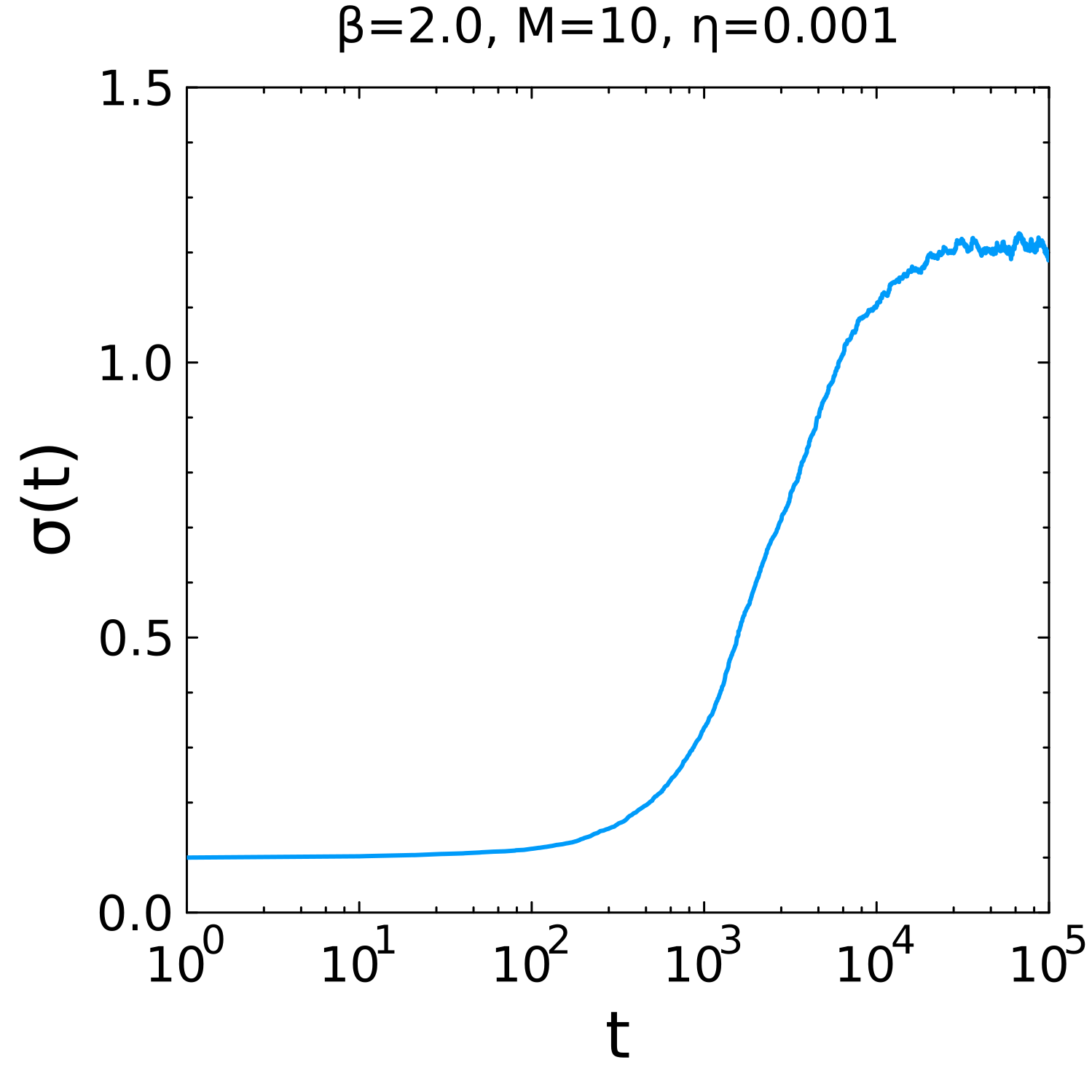
Standard deviation in function of time in a PGMC simulation.